Dynamic time warping
Dynamic time warping is a technique for manipulating time series data to enable comparisons between datasets, using local warping (stretching or compressing along the time axis) of the elements within each time series to find an optimal alignment between series. Unlike traditional distance measures such as Euclidean distances, the local warping in DTW can capture similarities that linear alignment methods might miss. By emphasising shape similarity rather than strict temporal alignment, DTW is particularly useful in scenarios where the exact timing of occurrences is less important for the analysis.
The DTW algorithm
Consider a time series to be a vector of some arbitrary length. Consider that we have \(p\) such vectors in total, each possibly differing in length. To find a subset of \(k\) clusters from within the total set of \(p\) vectors, where each cluster contains similar vectors, we must first make \(\frac{1}{2} {p \choose 2}\) pairwise comparisons between all vectors within the total set and find the `similarity' between each pair. In this case, the similarity is defined as the DTW distance between a pair of vectors. Consider two time series \(x\) and \(y\) of differing lengths \(n\) and \(m\) respectively,
\[x=(x_1, x_2, ..., x_n)\] \[y=(y_1, y_2, ..., y_m).\]The DTW distance is the sum of the Euclidean distance between each point and its matched point(s) in the other vector. The following constraints must be met:
- The first and last elements of each series must be matched.
- Only unidirectional forward movement through relative time is allowed, i.e., if \(x_1\) is mapped to \(y_2\) then \(x_2\) may not be mapped to \(y_1\) (this ensures monotonicity).
- Each point is mapped to at least one other point, i.e., there are no jumps in time (this ensures continuity).
Finding the optimal warping arrangement is an optimisation problem that can be solved using dynamic programming, which splits the problem into easier sub-problems and solves each of them recursively, storing intermediate solutions until the final solution is reached. To understand the memory-efficient method used in DTW-C++, it is useful to first examine the full-cost matrix solution, as follows. For each pairwise comparison, an \(n\) by \(m\) matrix \(C^{n\times m}\) is calculated, where each element represents the cumulative cost between series up to the points \(x_i\) and \(y_j\):
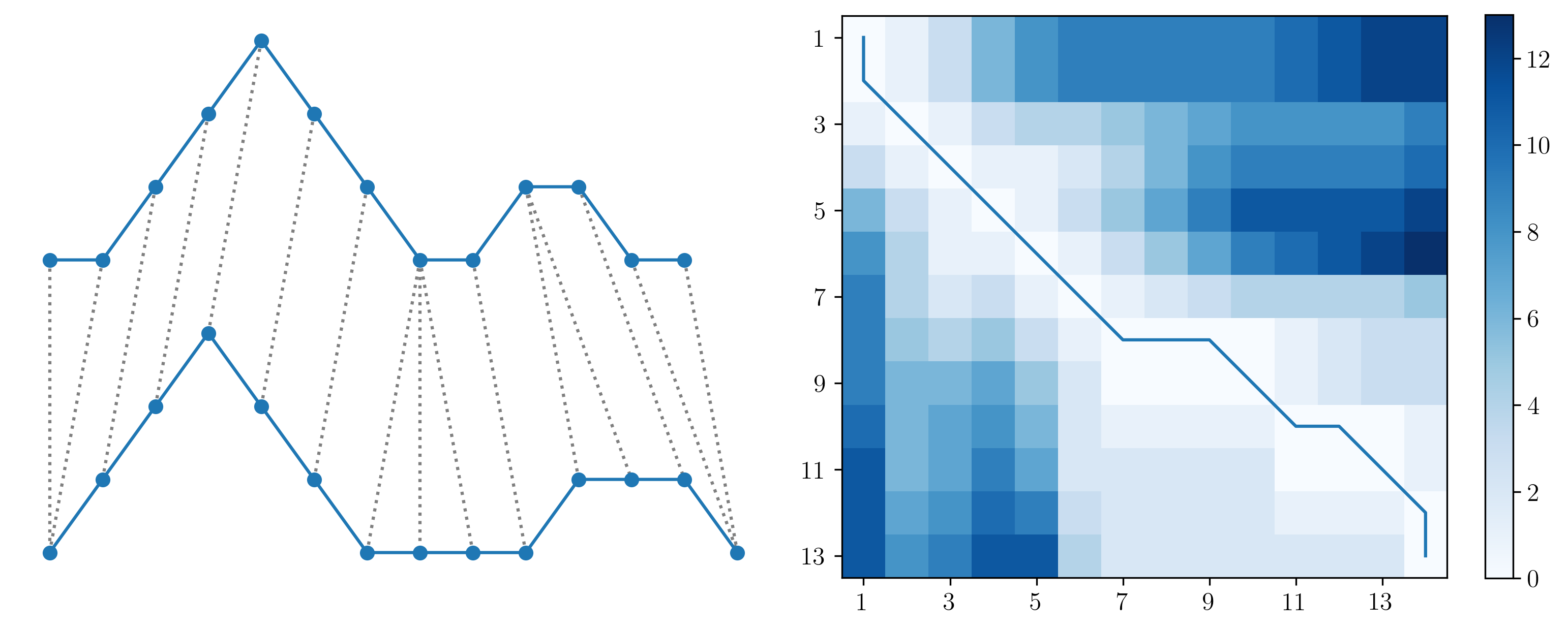
\[c_{i,j} = (x_i-y_j)^2+\min \begin{cases} c_{i-1,j-1}\\ c_{i-1,j}\\ c_{i,j-1} \end{cases}\]The final element \(c_{n,m}\) is then the total cost, \(C_{x,y}\), which provides the comparison metric between the two series \(x\) and \(y\). Below is an example of this cost matrix \(C\) and the warping path through it.
As an example, below are two time series with DTW pairwise alignment between elements. On the right is the cost matrix \(C\) for the two time series, showing the warping path and final DTW cost at element \(C_{14,13}\).
For the clustering problem, only the final cost for each pairwise comparison is required; the actual warping path (or mapping of each point in one time series to the other) is superfluous for clustering. The memory complexity of the cost matrix \(C\) is \(O(nm)\), so as the length of the time series increases, the memory required increases greatly. Therefore, significant reductions in memory can be made by not storing the entire \(C\) matrix. When the warping path is not required, only a vector containing the previous row for the current step of the dynamic programming sub-problem is required (i.e., the previous three values \(c_{i-1,j-1}\), \(c_{i-1,j}\), \(c_{i,j-1}\)).
In DTW-C++, the DTW distance \(C_{x,y}\) is found for each pairwise comparison. Pairwise distances are then stored in a separate symmetric matrix, \(D^{p\times p}\), where (\(p\)) is the total number of time series in the clustering exercise. In other words, the element \(d_{i,j}\) gives the distance between time series (\(i\)) and (\(j\)).
Warping Window
For longer time series it is possible to speed up the calculation by using a ‘warping window'. This works by restricting which data elements on one seies can be mapped to another based on their proximity. For example, if one has two data series of length 100, and a warping window of 10, only elements with a maximum time shift of 10 between the series can be mapped to each other. So, \(x_{1}\) can only by mapped to \(y_{1}-y_{11}\). Using a warping window of 1 results in clustering with Euclidean distances, forcing one-to-one mapping with no shifting allowed. The stricter the wapring window, the greater the increase in speed. However, the data being used must be carefully considered to assertain if this will negatively impact the results. Readers are referred Sakoe et al., 1978 for detailed information on the warping window.